But What Is a Neural Net? — Inspecting the 150-Line Training Loop
Karpathy builds a full neural-network training library from scratch — 150 lines of Python — then shows you every piece under the hood: the autograd engine, the expression graph, backpropagation, and the training loop.
Watch on YouTubeTL;DR
- micrograd does all of neural-network training in 150 lines
- backpropagation is just the chain rule, applied recursively backward through the computation graph
- gradients accumulate via += — the shared-node bug kills you if you use plain =
- you can bundle operations at any granularity (tanh, exp, power) as long as you know the forward and backward formulas
- the zero_grad() bug is the most common training mistake; gradients persist across iterations and corrupt the update
00 · The setup
The micrograd README
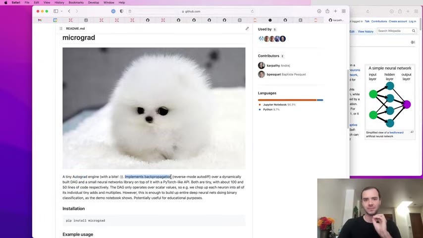
Karpathy introduces micrograd as a minimal autograd engine — "autograd" being short for automatic differentiation. His thesis: every neural network is just a mathematical expression, and training is differentiating the loss with respect to the weights and taking a step in the opposite direction. Everything beyond that — tensors, GPUs, batched ops — is efficiency.
"Fundamentally, all you need to train a neural net is a mathematical expression and back propagation." — Andre Karpathy
08 · Derivatives
Sensitivity, not symbols
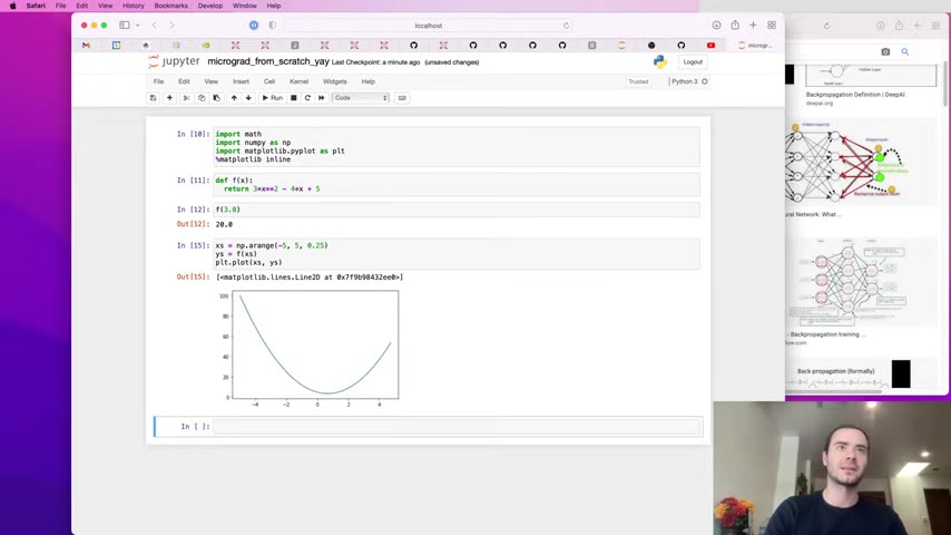
Before building any machinery, he establishes the intuition: a derivative measures how sensitive the output is to a tiny nudge in one input. He uses the numerical formula:
(f(x + ε) − f(x)) / ε where ε = 0.001
For a multi-variable function like d = a × b + c, each partial derivative tells you which input matters most:
∂d/∂a = b = −3— a has a strong negative influence∂d/∂b = a = 2— b pushes the output up∂d/∂c = 1— c's influence is unit-size
The sign tells direction; the magnitude tells strength. That's all gradient descent needs.
19 · The Value class
Building the expression graph
The Value class wraps a scalar and tracks its provenance:
class Value:
    def __init__(self, data, _children=(), _op=''):
        self.data = data
        self.grad = 0.0
        self._prev = set(_children)
        self._op = _op
Every + and * creates a new Value whose _prev points to its children and whose _op records the operation. This builds a directed acyclic graph of the forward pass — and the graph is all backpropagation needs to walk backward.
Python's operator overloading (__add__, __mul__, __rmul__, __pow__) means expressions read naturally: a * b + c.
29 · Back propagation
The chain rule in action
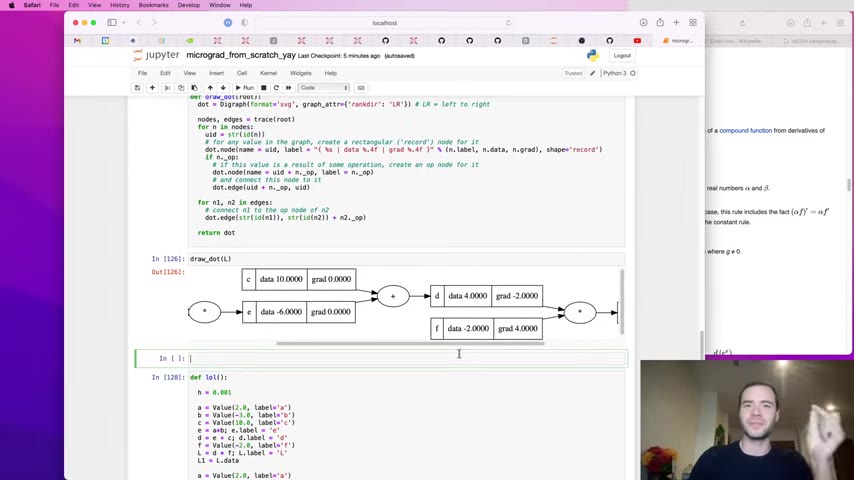
val and grad — the gradient flowing backward through the chain rule.00:38:14Backpropagation starts at the output node with grad = 1.0 and walks backward through the graph:
- Addition nodes split the gradient equally to both children (local derivative = 1)
- Multiplication nodes scale by the other input:
∂(x·y)/∂x = y - Composite nodes (tanh, exp, power) use their own local derivative
The chain rule compounds: ∂L/∂x = (∂L/∂y) · (∂y/∂x). Each node only knows its local derivative; the global gradient arrives from downstream and gets multiplied through.
"Knowing the instantaneous rate of change of z with respect to y and y relative to x allows one to calculate the instantaneous rate of change of z relative to x as a product of those two rates of change." — Chain rule intuition, via Wikipedia (cited in-video)
53 · Automating backward
Topological sort + the accumulation bug
The key insight: call backward() on every node in reverse topological order. The topological sort guarantees that when you visit a node, all of its children have already computed their gradients.
def backward(self):
    topo = []
    visited = set()
    def build_topo(node):
        if node not in visited:
            visited.add(node)
            for child in node._prev:
                build_topo(child)
            topo.append(node)
    build_topo(self)
    self.grad = 1.0
    for node in reversed(topo):
        node._backward()
The accumulation bug: if a variable appears more than once in the graph, = overwrites the gradient instead of adding to it. The fix is +=:
# Bug: self.grad = local * out.grad    # overwrites on shared nodes
# Fix:  self.grad += local * out.grad   # accumulates correctly
1:27 · Composite operations
tanh, exp, power
You can implement operations at any granularity — from atomic +/* to a bundled tanh — as long as you know the forward and backward formulas:
tanh(x)— backward:(1 − tanh²(x)) · gradexp(x)— backward:exp(x) · gradx ** k— backward:k · x^(k-1) · grad(power rule)
Division is just multiplication by x⁻¹: a / b = a * b ** (-1).
"As long as you know how to differentiate through any one function … that's all you need."
1:39 · PyTorch
Same API, bigger tensors
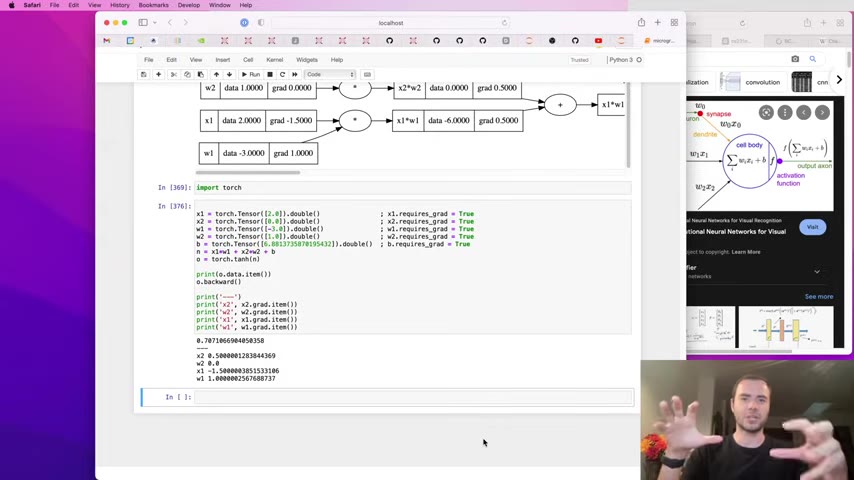
micrograd is intentionally designed to mirror the PyTorch API using single-element tensors:
| micrograd | PyTorch |
|---|---|
Value(2.0) |
torch.tensor(2.0, requires_grad=True) |
a + b |
a + b (identical) |
o.backward() |
o.backward() (identical) |
o.data |
o.item() |
a.grad |
a.grad (identical) |
The only difference is scale: production libraries use n-dimensional tensors to exploit GPU parallelism. The math doesn't change.
1:44 · Training
From neurons to gradient descent
Building a neural net from the ground up:
class Neuron:
    def __call__(self, x):
        act = sum(w_i * x_i for w_i, x_i in zip(self.w, x)) + self.b
        return act.tanh()

class Layer:
    def __call__(self, x):
        return [n(x) for n in self.neurons]

class MLP:
    def __call__(self, x):
        for layer in self.layers:
            x = layer(x)
        return x[-1]
Training loop (gradient descent, 100 steps, lr = 0.05):
for k in range(100):
    yhat = n(x)                       # forward
    loss = sum((ygt - yhat_i)**2 for ygt, yhat_i in zip(y, yhat))  # MSE
    n.zero_grad()                     # ← critical
    loss.backward()                   # backward
    for p in n.parameters():
        p.data -= 0.05 * p.grad       # update
Loss drops from ~7 → ~0.04 → near-zero. The network learns to classify the four training examples.
2:10 · The bug
Forgetting to zero_grad
Karpathy catches a real bug on camera: forgetting to call zero_grad() before each backward pass. Gradients accumulate across iterations (+= is additive by design), so the second forward pass starts with stale gradient values from the first.
The funny part: on this trivially simple problem, the corrupted gradients accidentally made convergence faster — the network happened to land in a good spot. On any real problem, this bug breaks training silently.
"You forgot to zero_grad before that backward."
2:14 · Recap
All you need
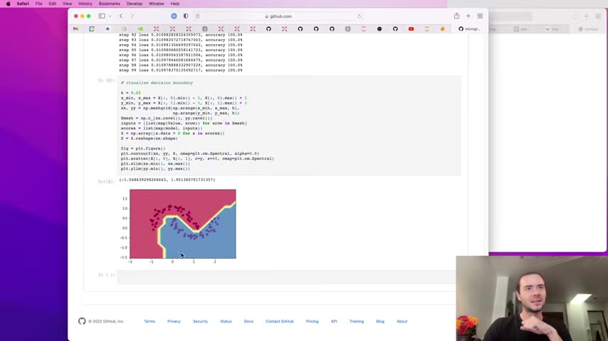
The complete picture:
- Forward pass — a mathematical expression takes data + weights → predictions
- Loss — a single number measuring how far predictions are from targets
- Backward pass — differentiate loss w.r.t. every weight via the chain rule
- Update — nudge every weight in the opposite direction of its gradient
- Repeat — gradient descent iterates steps 1–4 until the loss is low enough
micrograd distills this to scalar operations for clarity. GPT and every other modern model work on the exact same principles — just with billions of parameters, cross-entropy loss, and tensors on GPUs.
Forward pass is the expression; backward pass is the chain rule running backward through it
Gradients accumulate — use +=, never =
zero_grad() before every backward pass — the most common training bug
Abstraction level is a choice — bundle operations freely as long as you know forward + backward
Everything else is efficiency — tensors, GPUs, batched ops don't change the math
:::