Introduction to Quantum Computing

01 · Why quantum computing matters

Intro

Most explanations of quantum computers lean on analogies — "bits are both zero and one at the same time" — that don't land. This course skips the analogies and teaches the actual math: complex numbers, matrices, and vector rotations. The result is a foundation you can use to derive every quantum algorithm from first principles.

When I first started learning about quantum computers, these analogies and explanations never made sense. This course was created to provide a solid foundation without them.— Michael

02 · The math foundation

Imaginary & complex numbers

Quantum mechanics uses complex numbers in exponential form as its native language. Before getting to qubits, you need to understand why: rotating a quantum state is multiplication by $e^{i\theta}$, and that's what gives quantum gates their power.

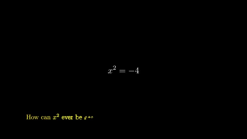
Any number that contains a factor of the square root of minus one, or $i$, is an imaginary number.— Michael

The course derives Euler's formula naturally — not as a fact to memorize but as the bridge between algebra and geometry. When both complex numbers have unit magnitude, multiplying them adds their angles, which maps directly to rotating on the unit circle.

03 · The math foundation

Matrices as transformations

Quantum operations are matrices. But not just any matrices — unitary matrices, which preserve vector length (rotations and reflections). The course also introduces Hermitian matrices, which appear in observable measurements.

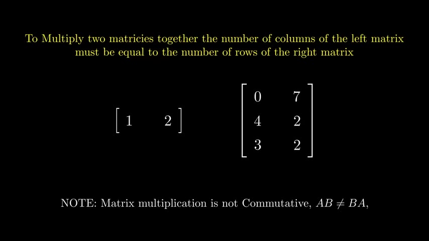
A unitary matrix $U$ satisfies $U^\dagger U = I$, meaning its conjugate transpose is its inverse. Geometrically, this means the matrix rotates or flips vectors without stretching them — essential because quantum probabilities must always sum to one.

04 · The qubit

What is a qubit?

A classical bit is 0 or 1. A qubit is a column vector $\begin{bmatrix}\alpha \ \beta\end{bmatrix}$ where $|\alpha|^2 + |\beta|^2 = 1$. The state $|0\rangle = \begin{bmatrix}1 \ 0\end{bmatrix}$ and $|1\rangle = \begin{bmatrix}0 \ 1\end{bmatrix}$ are the basis states in Dirac notation (bras and kets).

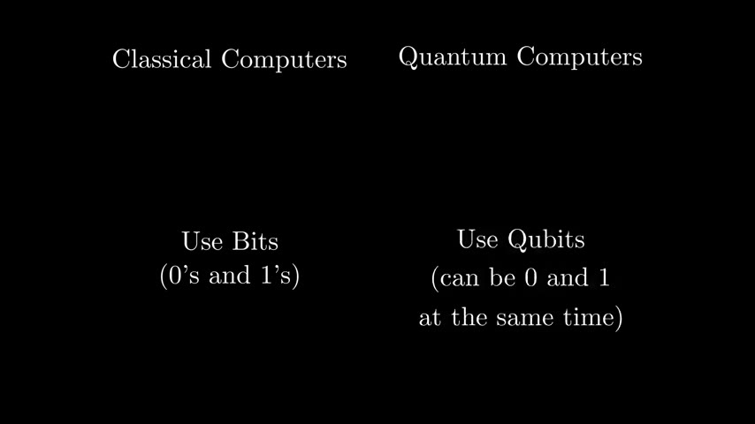
A qubit is in superposition if it has nonzero numbers in both the zero and one state — it is both of the states at the same time.— Michael

Measuring a qubit collapses its superposition: you get 0 with probability $|\alpha|^2$ and 1 with probability $|\beta|^2$, and the qubit permanently becomes that outcome. The numbers in the vector aren't the probability — their magnitudes squared are.

05 · Visualization

The Bloch sphere

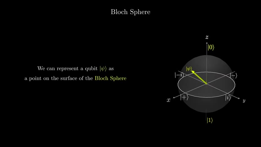
Any single-qubit state can be visualized as a point on a sphere. The north pole is $|0\rangle$, the south pole is $|1\rangle$, and the equator holds states with equal probability of measuring 0 or 1, differing only by phase.

06 · Quantum gates

Single-qubit gates

Quantum gates rotate the qubit state on the Bloch sphere. The X, Y, and Z gates each rotate 180° (π radians) around their respective axes. The Hadamard gate maps $|0\rangle$ to the plus state and $|1\rangle$ to the minus state.

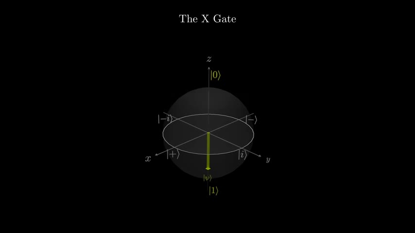
These three gates are their own inverses — applying the same gate twice returns the qubit to its original position.— Michael

The Z gate is subtle: it doesn't change measurement probabilities at all. It only adds a relative phase to the $|1\rangle$ component, multiplying it by −1. On the Bloch sphere, it rotates around the Z axis, which doesn't change the latitude (probability) but changes the longitude (phase).

07 · Phase

Hadamard & phase gates

Phase is what makes quantum computers powerful. The course distinguishes two types: global phase (physically irrelevant) and relative phase (extremely important). The S gate adds $\pi/2$ phase; the T gate adds $\pi/4$.

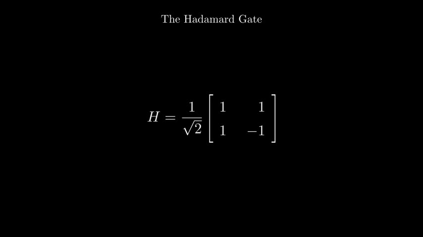
The Hadamard gate demonstrates why phase matters: $|+\rangle$ and $|-\rangle$ differ only by relative phase, but after another Hadamard they become $|0\rangle$ and $|1\rangle$ — different measurement outcomes from a difference that was invisible to direct measurement.

08 · Multi-qubit systems

Entanglement

Multiple qubits are represented by the tensor product of their states. A 2-qubit system has 4 basis states ($|00\rangle, |01\rangle, |10\rangle, |11\rangle$). When the joint state can't be factored into individual qubit states, the qubits are entangled — measuring one instantly determines the other.

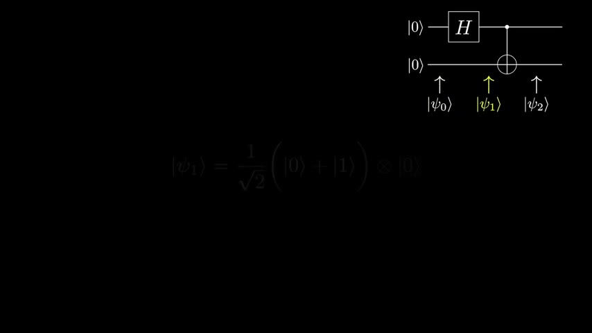
Without even looking at both the qubits, by measuring one of them we immediately know the state of the other qubit. This is called entanglement.— Michael

The course covers maximally entangled Bell states and partially entangled states, where measuring one qubit shifts the probabilities of the other without fully determining it.

09 · Protocol

Superdense coding

Superdense coding uses one pre-shared entangled qubit pair to transmit two classical bits by sending only one qubit. Alice applies one of four operations (identity, X, Z, or XZ) to her qubit, then sends it to Bob. Bob performs a Bell measurement to recover both bits.

10 · Algorithm

Deutsch's algorithm

Deutsch's algorithm is the simplest quantum speedup demonstration. Given a "black box" function that takes one bit and returns one bit, determine whether it's constant (always returns the same output) or balanced (returns 0 for one input, 1 for the other).

Classically, this requires two queries. Quantum mechanically, one query suffices. The algorithm uses a phase oracle: when the output qubit is in the $|-\rangle$ state, querying $f$ applies a relative phase of $(-1)^{f(x)}$ to the input qubit. A final Hadamard gate converts this phase difference into a measurable bit flip.

11 · Algorithms deep

Deutsch-Jozsa, BV, QFT & phase estimation

The course extends Deutsch's algorithm to n bits (Deutsch-Jozsa), then to finding a secret string (Bernstein-Vazirani). The quantum Fourier transform encodes numbers into the phases of superposition states, and quantum phase estimation extracts eigenvalues of unitary operators. These are the building blocks of Shor's factoring algorithm.

1. Step 1 — Choose $a$ coprime to $n$ (the number to factor)
2. Step 2 — Use quantum phase estimation to find the period $r$ of $a^x \bmod n$
3. Step 3 — Use continued fractions to estimate $s/r$ from the measured phase
4. Step 4 — Compute $\gcd(a^{r/2} \pm 1, n)$ to find the factors

We will need a fault-tolerant quantum computer with millions of logical qubits — which won't happen for some time. But the algorithm shows that quantum computers can factor large numbers exponentially faster than any known classical method.— Michael